Optimal Localization of Postal Offices

Poste Italiane – Spatial Optimization & Location-Allocation

Project status: this work was initiated in collaboration with, and at the suggestion of, Poste Italiane as an exploratory case study, but it did not reach a final deployed stage. It is not an official Poste Italiane product, and figures, screenshots, and simulation data shown here should be read as work-in-progress / illustrative rather than production results.

An end-to-end analytical framework combining Mixed-Integer Linear Programming (MILP), geocoding pipelines, and dynamic scenario modeling for postal facility placement and customer drift simulation.

Post offices (UP – Ufficio Postale) form the vital backbone of Italy’s physical service ecosystem. When a post office closes or shifts capacity, the ripple effect triggers a spatial realignment of customer flows, revenue reallocation, and migration toward partner networks (such as LIS – Punto LIS), digital channels, or commercial competitors.

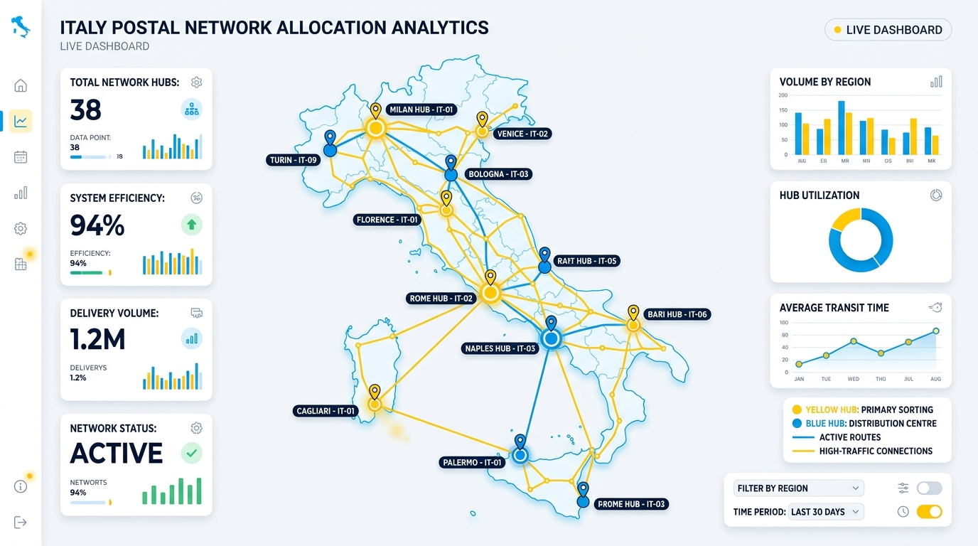
12,800+

Post Offices (UP) Processed

50,000+

LIS Partner Points

< 100ms

Re-allocation Solver Speed

100%

Postal Code Validation

Solver speed and validation figures are benchmark-specific — see Assumptions & Limitations for methodology.

The Operational Challenge

When evaluating network optimizations or branch closures, customer service demands are categorized according to their transaction characteristics and re-allocation pathways:

Service Category	Re-allocation Pathway	Customer Flow Dynamic
Over-The-Counter Transactions (Bollettini, PagoPA, MAV, Postepay recharges, SIM card top-ups, Parcel drop-offs)	Partial migration to nearby LIS points and adjacent UPs.	Customers divide between local proximity options, digital shifts, and competitor retention/loss.
Financial & Insurance Products (Polizze, Libretti, Financial Accounts, Energy & Telecom contracts)	Shift primarily to surrounding full-service UPs within target travel radius.	Higher friction sensitivity; requires spatial accessibility modeling based on population density.

Optimization & Data Pipeline Schema

System workflow from raw address ingestion to linear optimization and scenario map rendering:

01. Normalization

Italian address parsing, street type standardizing, postal code validation (CAP).

02. Geocoding

Rate-limited OpenStreetMap API resolution with cache fallback and spatial projection.

03. MILP Solver

Location-Allocation linear programming optimizing distance matrices vs capacity constraints.

04. Interactive Map

PosteScope web simulator & Folium map rendering for decision-maker what-if scenarios.

Mathematical Formulation

The location-allocation optimization models facility positioning and demand point assignment as a Mixed-Integer Linear Program (MILP) implemented in Python via PuLP.

Objective Function (Minimize Total Travel Distance)

$$\min \sum_{i \in \text{Demand}} \sum_{j \in \text{Facilities}} d(i, j) \cdot y(i, j)$$

1. Demand Coverage Constraint

$$\sum_{j \in \text{Facilities}} y(i, j) = 1 \quad \forall i \in \text{Demand}$$

Guarantees that every demand node i is assigned to exactly one facility.

2. Facility Activation Constraint

$$y(i, j) \le x(j) \quad \forall i \in \text{Demand}, \, j \in \text{Facilities}$$

Prevents assignment of demand to closed or inactive post offices.

3. Facility Upper Bound

$$\sum_{j \in \text{Facilities}} x(j) \le P$$

Restricts total active facilities to a maximum target threshold P.

4. Binary Decision Variables

$$x(j) \in \{0, 1\}, \quad y(i, j) \in \{0, 1\}$$

Strict integer requirements enforcing open/close and assignment decisions.

5. Facility Capacity Constraint

$$\sum_{i \in \text{Demand}} w(i) \cdot y(i, j) \le c(j) \quad \forall j \in \text{Facilities}$$

Caps demand volume assigned to each open facility at its service capacity, preventing overload and forcing genuine overflow to LIS points and adjacent UPs.

Notation Legend:

d(i, j): Distance/time matrix between demand i and facility j
x(j): Binary variable (1 if facility j is open, 0 otherwise)
y(i, j): Binary variable (1 if demand i is assigned to facility j)
w(i): Transaction volume/weight of demand node i
c(j): Service capacity of facility j

Assumptions & Limitations

The facility-selection MILP was designed but not implemented in the current prototype. The location-allocation formulation above (minimizing total distance subject to coverage, activation, capacity, and cardinality constraints) describes the intended model for choosing which facilities to open or close under a target count P. The working prototype does not run this solver — closures are specified manually (one UP at a time), not selected by optimization.
Redistribution uses an implemented distance-weighted gravity model. Once a closure is specified, affected demand is redistributed to nearby UPs, LIS points, and competitors using inverse-distance-squared weighting, with catchment radii that adapt to local population density (rural, suburban, urban, high-density) and per-service redistribution coefficients (e.g., parcels vs. financial products split differently). This part of the pipeline is real and was implemented.
Solver speed. The <100ms figure describes the gravity-model redistribution calculation for a single closure, not a MILP solve — no MILP solver runs in the current prototype (see above).
Data. Some pipeline runs use synthetic/randomly generated UP, LIS, and bank locations for demonstration; the more advanced redistribution model is built to load real UP/LIS/bank/census/footfall data but was not run end-to-end on a full national dataset.
Postal code validation. The 100% figure covers CAP-format and address-parsing checks on ingested records, not positional geocoding accuracy, which varies with source data quality.
Distance metric. Distances are haversine/great-circle or straight-line approximations and do not yet incorporate real-time traffic or public transit schedules.

PosteScope Simulator Engine

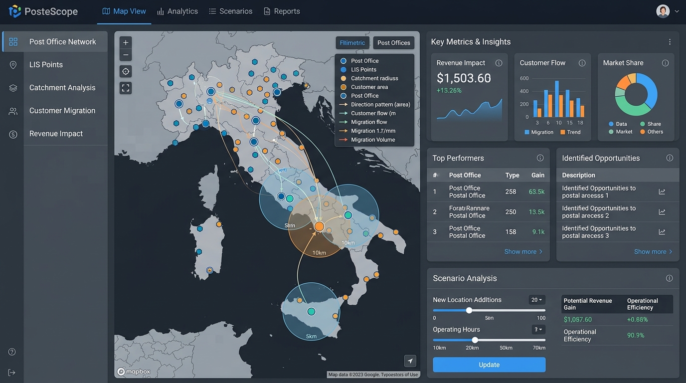PosteScope Interactive Scenario Simulator

Interactive What-If Simulation Capabilities:

Facility Closure Analysis: Select any UP to close and observe downstream production redistribution.
LIS Capacity Placement: Simulate adding new partner point locations to absorb transaction overflow.
Revenue & Churn Quantification: Live metric cards computing expected financial impact, digital channel shifts, and competitor capture ratios.
Density-Scaled Radii: Catchment buffer sizes dynamically adjust according to urban, suburban, and rural municipality classifications.

Live Geospatial Simulation Maps

Illustrative regional subset for walkthrough purposes — full production runs cover the 12,800+ UP national network.

Blue: Active Post Office (UP) Green: LIS Partner Point Red: Bank Branch

Click markers to inspect production metrics