Exploring precipitation time series with R and NASA Giovanni
This tutorial explores how to import precipitation time-series data from a .csv file into R, work with columns in a data.frame, and convert dates stored as character strings into a format that R can recognise and plot.
The data for this example were obtained through NASA Giovanni, a web application developed by the Goddard Earth Sciences Data and Information Services Center (GES DISC). Giovanni provides access to satellite observations and model outputs covering rainfall, atmospheric conditions, land surfaces and oceans. This walkthrough uses historical TRMM Multi-satellite Precipitation Analysis (TMPA) data.
Giovanni provides a convenient way to explore Earth observation data in a web browser. You can view maps and time series before downloading data, making it easier to identify a useful dataset and define the scope of an analysis.
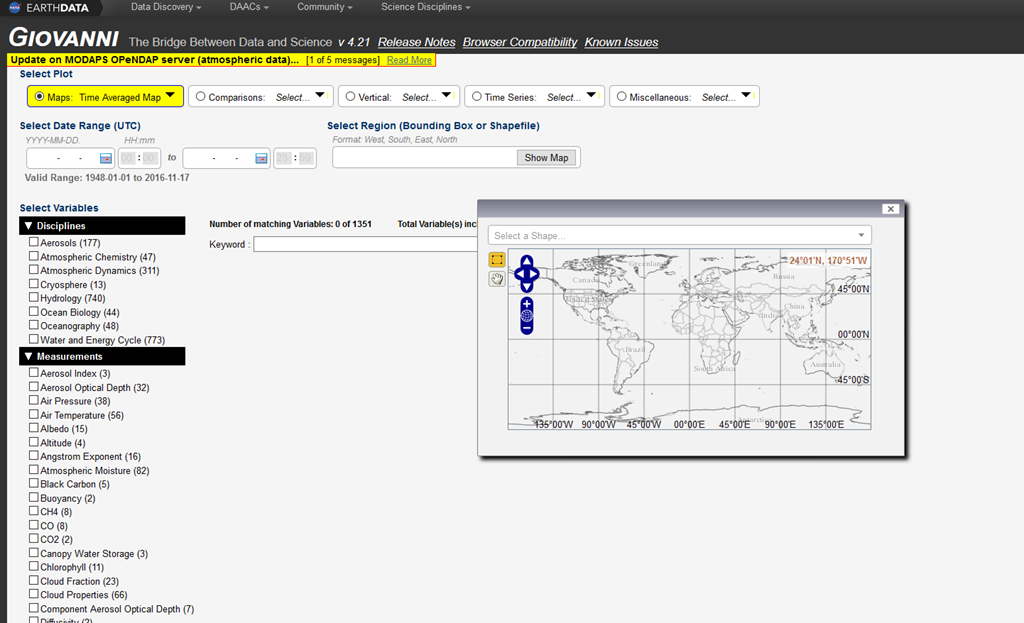
For this example, I selected the study area, time period, precipitation variable and output type in Giovanni. The interface allows a region to be defined using a bounding box. Results can be explored as plots or downloaded as text files for further analysis in R or GIS software. Processing time depends on the amount of data requested.
The screenshots below show the interface used for the original analysis.
The purpose of the 3B42 algorithm is to produce TRMM-adjusted merged-infrared (IR) precipitation and root-mean-square (RMS) precipitation-error estimates. The algorithm consists of two separate steps. The first step uses the TRMM VIRS and TMI orbit data (TRMM products 1B01 and 2A12) and the monthly TMI/TRMM Combined Instrument (TCI) calibration parameters (from TRMM product 3B31) to produce monthly IR calibration parameters. The second step uses these derived monthly IR calibration parameters to adjust the merged-IR precipitation data, which consists of GMS, GOES-E, GOES-W, Meteosat-7, Meteosat-5, and NOAA-12 data. The final gridded, adjusted merged-IR precipitation (mm/hr) and RMS precipitation-error estimates have a daily temporal resolution and a 0.25-degree by 0.25-degree spatial resolution. Spatial coverage extends from 50 degrees south to 50 degrees north latitude.
Strengths of the historical dataset
- Offers high spatial and temporal resolution precipitation estimates over a relatively long period of record (since 1998)
- Useful for investigating the climatological distribution of rainfall, including its frequency and intensity.
- Useful for validation of tropical precipitation in climate models, provided that care is taken to put the data on comparable grids using conservative re-gridding and to use accumulated (rather than instantaneous) precipitation
Limitations to consider
- Complex algorithms are required to translate indirect and infrequent satellite measurements into high-resolution gridded precipitation estimates at regular time intervals
- TRMM precipitation radar algorithm likely underestimates precipitation in (a) regions of intense convection over land and (b) higher latitudes
- As a Climate Data Record with global coverage, GPCP should be preferred over TRMM for large-scale climate variability studies
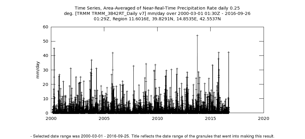
TMPA time series combine estimates from changing data sources, so the record may contain temporal inconsistencies. Each grid cell represents an estimate of precipitation at the observation time. TMPA was designed to provide detailed precipitation estimates and does not have the same homogeneity objectives as a climate dataset such as GPCP v2.2.
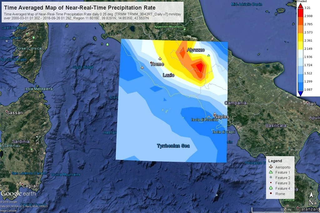
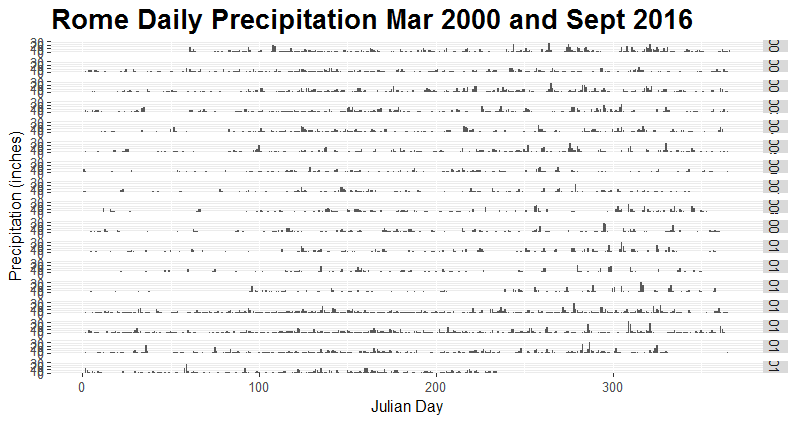
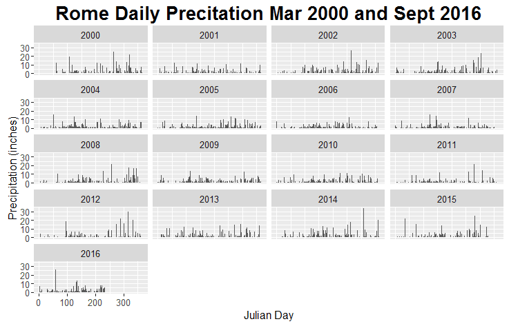
The example shown here uses Version 7 TMPA-RT data to map accumulated rainfall in the Rome region over 2000–2016. Giovanni outputs can be saved as images or exported as time-series data.
For the R analysis, I used .csv (comma-separated values) files. In this plain-text format, commas separate values and line breaks separate rows. CSV files are widely supported across operating systems and analytical tools.
Separating trend and seasonality
Seasonal and trend decomposition using Loess (STL) separates a time series into three components: trend, seasonality and remainder. The method was presented by Robert Cleveland, William Cleveland, Jean McRae and Irma Terpenning in 1990 and is available in R through the stl function.
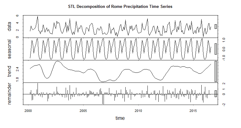
The four panels show the original observations, seasonal component, trend and remainder. The bars on the right help compare the scale of variation across panels. In this example, seasonal fluctuations are larger than changes in the underlying trend.
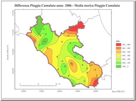
The trend component shows a pronounced rainfall deficit in 2006. Negative values in the remainder component also indicate periods with rainfall below the level explained by the trend and seasonal pattern.
The historical account cited in the original analysis described low rainfall and snowfall across Italy in 2006, alongside above-average temperatures. In Lazio, the deficit was particularly evident from September to December. Limited snow cover in the Apennines and observations from springs sensitive to precipitation raised concerns about reduced flows in the following months, with possible consequences for irrigation and minimum river flows. The account reported no critical problems with drinking-water supplies.
This walkthrough is based on historical TRMM-era data and screenshots. It illustrates a workflow for exploring rainfall and separating seasonal patterns from longer-term changes; the dataset and interface shown should be understood in that historical context.