Preliminary study
Predicting fall armyworm presence with machine learning
In December 2019, the Food and Agriculture Organization of the United Nations (FAO) launched the Global Action for Fall Armyworm Control in response to the rapid spread of fall armyworm (FAW). The initiative aimed to strengthen prevention and sustainable pest management through international coordination, national task forces and applied research.
FAO’s Fall Armyworm Monitoring and Early Warning System (FAMEWS) was developed to collect standardised field observations through a multilingual mobile application. Farmers, extension agents and other users can record observations while inspecting crops or checking pheromone traps. These records help describe infestation patterns and support pest management.
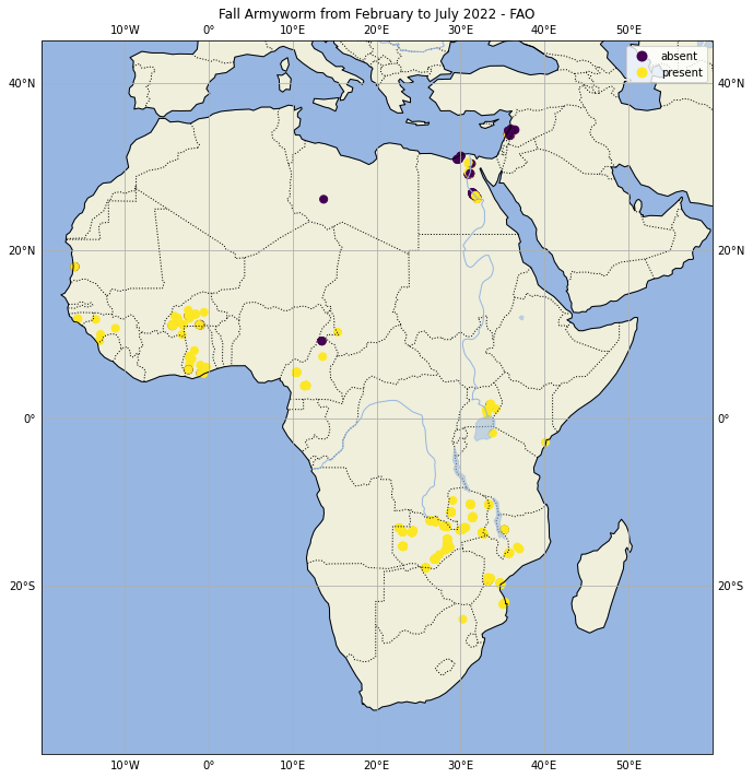
This preliminary study uses field observations made available through FAO’s Hand-in-Hand Geospatial Platform. The records used here include the number of plants inspected, the number found to be infested and the resulting infestation percentage.
The available observations are sparse and unevenly distributed. Records reporting FAW presence greatly outnumber those reporting its absence. These limitations are central to interpreting the analysis and its predictive results.
.png "image")
Adding environmental data to field observations
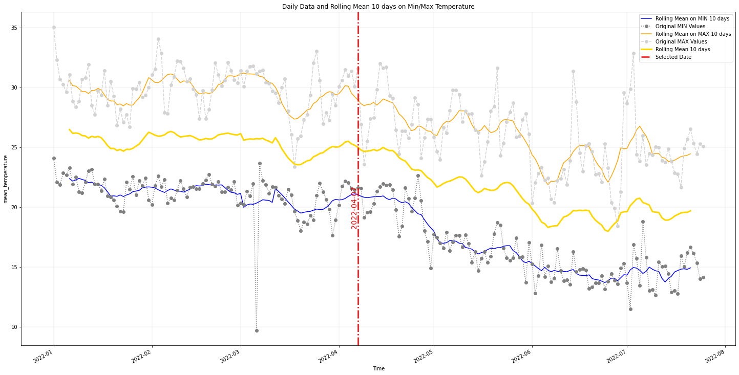
I used the latitude and longitude of each field observation to associate it with meteorological, soil-moisture and vegetation data. Some datasets were downloaded and processed locally; others were accessed through Google Earth Engine. Each field record was linked to ten days of environmental observations. The image below illustrates the resulting temperature time series.
CHIRPS Data Rainfall Estimates from Rain Gauge and Satellite Observations
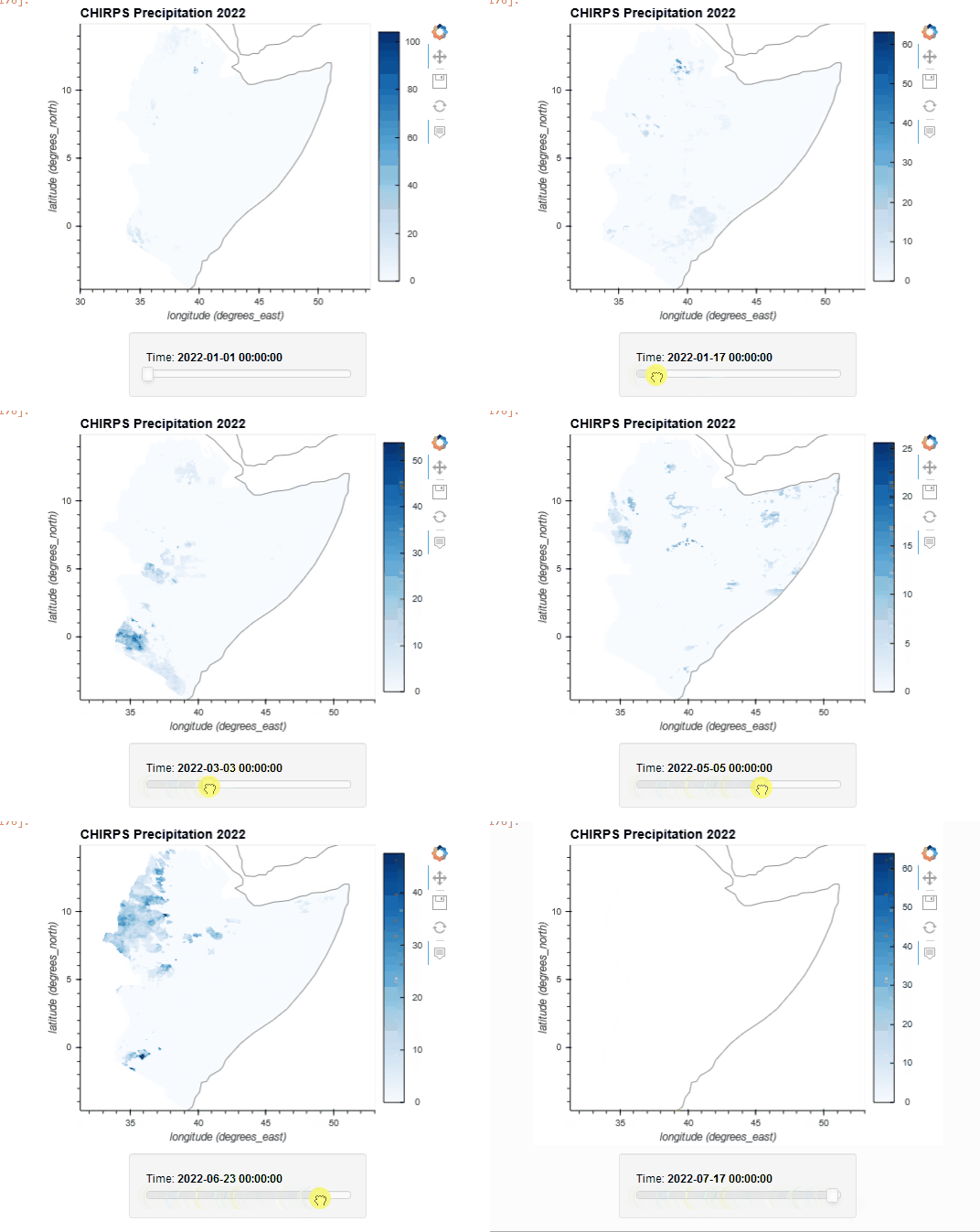
CHIRPS combines rain-gauge observations with satellite-based rainfall estimates. It provides a useful source of precipitation data for drought monitoring and seasonal analysis, particularly where ground observations are sparse.
Rainfall estimates still have limitations. Complex terrain can introduce bias in satellite estimates, while sparse rain-gauge coverage can reduce the reliability of station-based products in rural areas.
Temperature data
Temperature was included as an environmental predictor alongside rainfall, soil moisture and vegetation cover. The temperature time series associated with each field record provides context for the conditions around the observation date.
Soil Moisture from GLDAS-2.1: Global Land Data Assimilation System
The Global Land Data Assimilation System (GLDAS) combines satellite and ground observations with land-surface modelling to estimate land-surface conditions. This analysis uses GLDAS-2.1 root-zone soil moisture, represented by the RootMoist_inst variable and expressed in kg/m².
Fraction of green vegetation cover
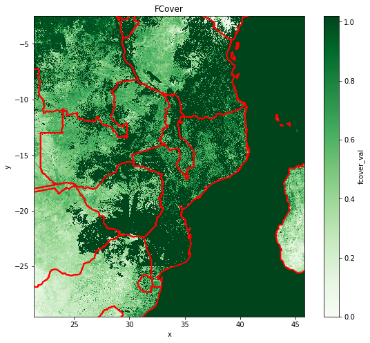
The fraction of vegetation cover (FCover) describes the fraction of ground covered by green vegetation. It provides a measure of vegetation extent that complements the weather and soil-moisture variables used in this study.
Exploratory Data Analysis
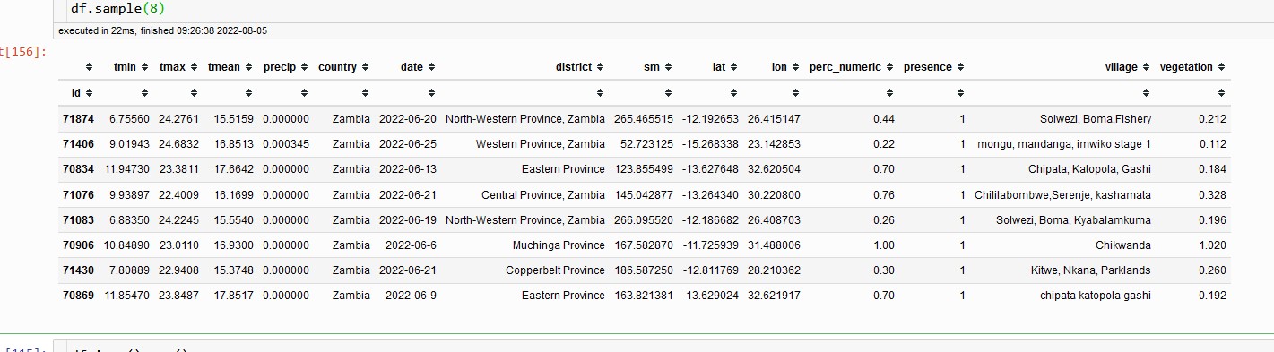
The enriched dataset combines environmental variables with a binary label indicating whether FAW was present or absent. Before modelling, I examined the added data and the relationships between predictors and pest observations.
The dataset contains 4,810 records: 4,410 labelled “present” and 400 labelled “absent”, a ratio of approximately 11:1. This class imbalance can favour predictions of the more common class and makes overall accuracy alone an inadequate measure of model performance.
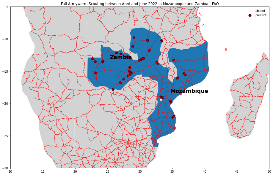
The observations cover only a small part of Africa and remain sparse even within individual countries. Many points appear to follow roads rather than represent more remote agricultural areas. Some are located in urban areas, where crop fields may be limited. These patterns raise questions about sampling coverage and location accuracy, and limit how confidently the results can be extended to other places.
According to CABI:
A threshold temperature of 10.9°C and 559 day-degrees C is required for development. Sandy-clay or clay-sand soils are suitable for pupation and adult emergence. Emergence in sandy-clay and clay-sand soils was directly proportional to temperature and inversely proportional to humidity. Above 30°C the wings of adults tend to be deformed. Pupae require a threshold temperature of 14.6°C and 138 day-degrees C to complete their development (Ramirez-Garcia et al., 1987). S. frugiperda is a tropical species adapted to the warmer parts of the New World; the optimum temperature for larval development is reported to be 28°C, but it is lower for both oviposition and pupation. In the tropics, breeding can be continuous with four to six generations per year, but in northern regions only one or two generations develop; at lower temperatures, activity and development cease, and when freezing occurs all stages are usually killed. In the USA, S. frugiperda usually overwinters only in southern Texas and Florida. In mild winters, pupae survive in more northerly locations.
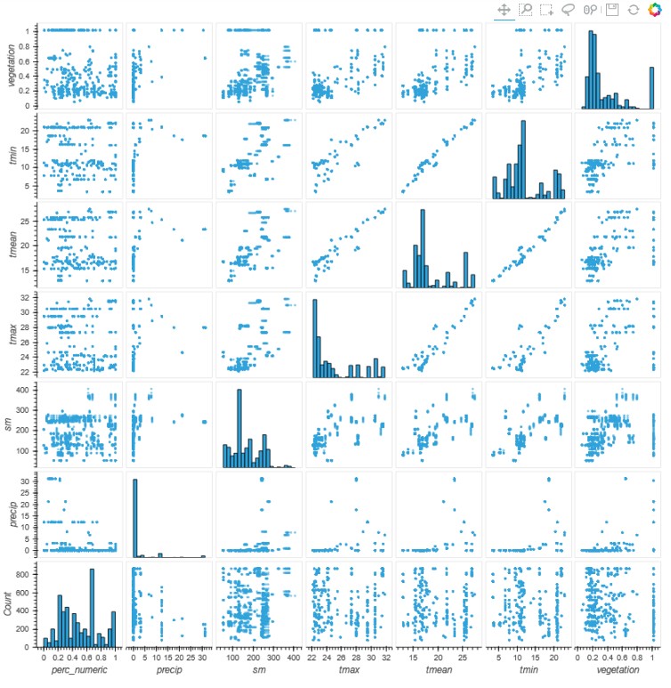
In this dataset, infestation levels show weak correlations with the temperature, soil-moisture, vegetation and precipitation variables examined. These observations alone do not establish which environmental factors drive FAW presence, particularly given the uneven sampling coverage.
Feature Engineering
- Feature Engineering Techniques Applied
- Feature Scaling
- Random undersampling
Feature scaling brings predictors measured in different units onto comparable numerical scales. Temperature, rainfall and soil moisture can have very different ranges; for some algorithms, these differences can affect fitting. Scaling helps address this issue during preprocessing. See the scikit-learn documentation for an example.
To reduce the imbalance, I used random undersampling to remove observations from the overrepresented class. The Python library imbalanced-learn provides tools for this process. Undersampling produces a more balanced dataset, but it also discards observations that may contain useful information.
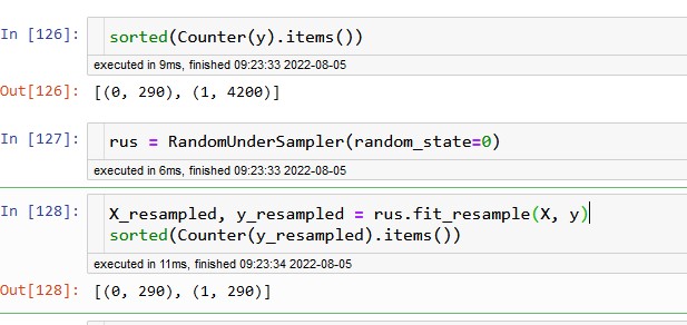
The sampler follows a scikit-learn-style interface:
fitdetermines the sampling strategy from the feature data and class labels.
fit_resampleapplies the strategy and returns the resampled feature data and corresponding labels.
For this study, I used RandomUnderSampler, which randomly selects a subset of observations from the targeted class. The imbalanced-learn documentation explains the method and its options.
Syntax:
from imblearn.under_sampling import RandomUnderSamplerExample: RandomUnderSampler(sampling_strategy="auto", replacement=False)
Implementation:
X_under, y_under = undersample.fit_resample(X, y)
The call returns two objects: X_under, containing the resampled features, and y_under, containing their class labels.
Logistic regression — approximately 78% accuracy
Logistic regression estimates the probability of an event from a set of predictor variables. Here, the event is FAW presence. The predicted probability lies between 0 and 1 and is converted into a class label using a decision threshold.
| precision | recall | f1-score | support | |
|---|---|---|---|---|
| absent | 0.88 | 0.65 | 0.75 | 57 |
| present | 0.73 | 0.92 | 0.81 | 59 |
| accuracy | 0.78 | 116 | ||
| macro avg | 0.81 | 0.78 | 0.78 | 116 |
| weighted avg | 0.80 | 0.78 | 0.78 | 116 |
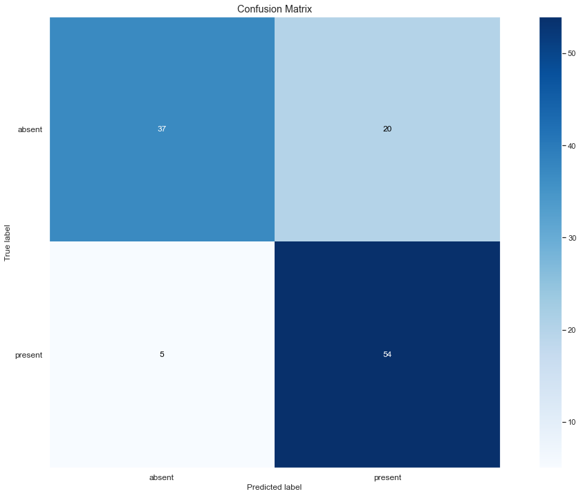
The classification report covers 116 observations: 57 with FAW absent and 59 with FAW present. The reported recall values correspond to 37 correctly classified absence records and 54 correctly classified presence records. There were 20 false positives and 5 false negatives, treating FAW presence as the positive class.
Changing the default probability threshold of 0.5 changes the balance between false positives and false negatives. The appropriate threshold depends on the purpose of the prediction and the consequences of each type of error.
Conclusions
The classification report shows an overall accuracy of approximately 78%. For FAW presence, precision is 73% and recall is 92%: the model identifies most presence cases in this evaluation, but some absence cases are incorrectly labelled as present.
Precision is the proportion of predicted presence cases that are correct. Recall is the proportion of actual presence cases that the model identifies.
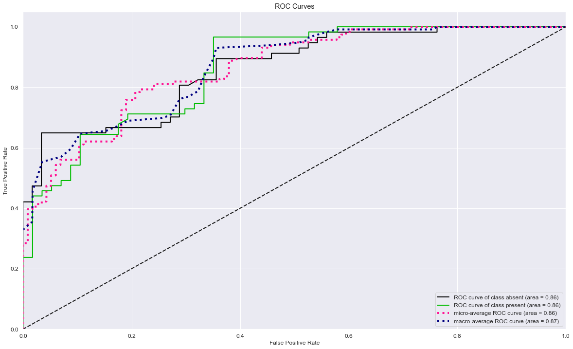
These are preliminary results from a small evaluation sample. The original class imbalance, loss of observations through undersampling and uneven geographic coverage limit the conclusions that can be drawn about performance elsewhere. The ROC curve below illustrates the trade-off between true-positive and false-positive rates across decision thresholds.